Piet Lammertse on propeller theory

VORTEX THEORY

23 The propeller lifting line

23.1 The spiral horseshoe vortex

The vortex field around a propeller is more complicated than that around a wing, but the principle is the same.

Figure 23.1 shows the "horseshoe" vortex from a single propeller blade. It is the equivalent of the single horseshoe on the wing of figure 21.3, but it looks even less like one...

This simplest of propeller lifting line models is sometimes called the "Joukowsky" rotor.

Figure 23.1 : Joukowsky rotor : core, bound, and tip vortex of a single "horseshoe".

Both the bound vortex and the root vortex ( i.e. the inner tip vortex ) are straight lines, just like in the wing. However, the outer tip vortex follows the spiral path of the blade tip.

The frontispiece photograph of a Hawker Hurricane ticking over on a moist day, shows that these spiral vortices are more than just a theoretical model.

We will develop this horseshoe spiral model first into a justification for the ideal actuator disk, and then into a tip loss and lifting line model for propellers of finite tip speed ratio.

23.2 The thrust from the bound vortex

First we have a look at the thrust. Like in the wing, and for the same reasons, the thrust comes exclusively from the bound vortex. The core vortex and the spiral vortex drift with the flow, and therefore they cannot generate thrust, or any other force.

The vortex lift (21.3) , alias the Lorentz force, on a blade element of spanwise width dr generates both the torque and the thrust for that element. The Lorentz force works at right angles to the flow, and since it is linear in the velocity, it can be split into two orthogonal components. The axial component V of the local airspeed relative to the blade gives a tangential force at right angles to it. This leads to a torque, but we will not be using the torque directly in our derivations.

The tangential velocity Ω r gives an axial force, or in other words a thrust, on the blade element. From the generic Lorentz force (21.3), this axial thrust is :

d T = ρ . Ω r . Γ . d r;

(23.1)

At any given Ω, the thrust on a blade element is proportional to the local radius r. But so is the ring area 2π r . dr swept by that element. For a single bound vortex, the thrust per frontal area is therefore constant over the whole prop disk.

The overall thrust follows by integrating (23.1) over the blade span for the single constant value of Γ :

T = \int_{0}^{R} ρ . Ω r . Γ . d r = ½ ρ . Ω R^{2} . Γ

(23.2)

23.3 The non-dimensional thrust

We can make the thrust non-dimensional by the definition of (3.2) :

T ′ = \frac{½ ρ . Ω R^{2} . Γ}{ρ V^{2} . π R^{2}} = \frac{1}{2π V} . \frac{Ω}{V} . Γ

(23.3)

Multiplying by R top and bottom and using X = Ω R / V from (2.11) we get :

T ′ = \frac{Γ . X}{2π R . V}

(23.4)

In the propeller, we will define a non-dimensional vortex strength Γ ′ :

Γ ′ \equiv \frac{Γ}{2π R . V}

(23.5)

This changes (23.4) to :

T ′ = Γ ′ . X

(23.6)

The factor X is a bit unexpected at first, but it derives from the decision to use the thrust ( and not the torque ) as the basic design parameter. This makes it more appropriate to use V as the reference velocity, and not Ω R.

The next section discusses the interpretation of the factor X further.

23.4 Axial induction in the ideal propeller

For the axial induction, we will first look at the " ideal" case of very flat spirals, i.e. for spirals of "infinitely small pitch". Like for the Lorentz force (22.3), there is a direct electro-magnetic equivalent. This is the tightly wound electrical coil, the so-called "solenoid".

Figure 23.2 gives a schematic impression. A wire carrying an electrical current is wound as a coil around a passive empty tube, and this generates a magnetic field inside the tube. It turns out that the magnetic field becomes parallel and uniform inside the coil, and zero outside it.

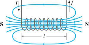
Figure 23.2 : Magnetic field lines inside and outside a solenoid.

We are going to use the solenoid as an analog for the spiral vortices wound around a flow tube. The transformation between the electromagnetic and the aerodynamic domains is :

Γ ↔ μ_{o} . I

(23.7)

v ↔ B

(23.8)

If s is the axial spacing between the spirals or coils, then the axial induction inside a tightly wound "tip" spiral is :

w = \frac{Γ}{s}

(23.9)

The direct derivation by the law of Biot-Savart is relatively straightforward, but we will take the result for granted here. It can be looked up in any text on electrical ( potential ) theory.

In the propeller, by figure 2.4 the tip spacing equals 1 /X times the prop disk circumference 2π R :

s = \frac{2π R}{X}

(23.10)

Substituting this into (23.9) V yields :

w = \frac{Γ}{2π R} . X

(23.11)

Dividing by V, by (23.5) the non-dimensional version is :

\frac{w}{V} = \frac{Γ}{2π R . V} . X = Γ ′ . X

(23.12)

With (23.6) we have :

\frac{w}{V} = T ′

(23.13)

With (4.2), this result is identical to (5.10) for the ideal actuator disk. Like in the elliptical wing with uniform downwash, the vortex picture gives a "physical" justification for the actuator tube flow with a uniform propwash inside the tube, and zero outside it.

The factor X reflects the fact that the thrust on the bound vortex is proportional to the ( tip) circumferential velocity, which is a factor of X larger than the axial velocity. The same thrust can be generated by narrow-chord blades turning at high RPM, or by wider chord blades turning at lower RPM. This is the interpretation from the bound vortex.

We can also make sense of the factor of X via the trailing spirals. In the electrical solenoid, the same magnetic induction can be generated by many windings of thin copper wire carrying a small current, or by fewer windings of thicker wire carrying a larger current. They will have the same "current density per length" ( known in the electrical world as " Ampère turns" per length ).

Similarly, we can see the Γ ′. X in (23.12) as the "vortex density per length" on the surface of the flow tube. This vortex density determines the axial induction inside the tube.

23.5 Mass flow in the ideal propeller

By (23.1) we know that the thrust is uniform over the prop disk and zero outside it. By (23.11) we know that the axial induction is uniform on the prop disk, and again zero outside it. This means that the Joukowsky rotor with infinitesimally small pitch is identical to the ideal actuator disk of figure 4.1, with uniform thrust and uniform induction inside a closed tube.

Combining the overall thrust (23.2) with the induction (23.11) allows us to find the effective mass flow. From Newton's law (4.7) we have :

m^{•} = \frac{T}{w} = ½ ρ . Ω R^{2} . Γ . \frac{2π R}{Γ . X} = \frac{ρ π . Ω R^{3}}{X}

(23.14)

With X ≡ Ω R / V this simplifies to :

m^{•} = ρ V . π R^{2}

(23.15)

This matches exactly with equation (5.2), which simply assumed that the effective mass is the mass ρ V flowing through the actuator disk frontal area π R².

It is also strikingly similar to (21.22) for the ideal wing. But most importantly, the solenoid model provides the "physical" justification for the ideal actuator disk model, with its sharp edge between the uniform, full induction inside the tube and zero induction outside it.