VORTEX THEORY
The elliptical wing from the previous chapter is an idealization. It is not normally realized in practical wings, and especially not in off-design conditions. This chapter describes a more general theory, but still based on the idea of simple horseshoe vortices.
Since potential theory for small deflection angles is a linear theory, an arbitrary wing can be interpreted as an in place superposition of simpler wings, of varying span and shape. Prandtl therefore was able to model the real wing as a collection of horseshoes of different spans, all centered at the same lifting line.
We discuss two ways of assembling a consistent lift and downwash distribution from a collection of horseshoe vortices : the analytical Fourier method, and the discrete method. Prandtl and Glauert both used the Fourier method. We will briefly discuss it, and then move on to the more "brute force" discrete method.
In both cases, the calculation for the lift distribution fitting an arbitrary wing shape is iterative. A lift or bound vortex distribution is first assumed, maybe starting with the physical wing planform as a first estimate for the shape. The trailing vortices are the changes in the bound vortex, or in analytical terms, its derivative.
The downwash at the wing is then calculated from the trailing vortices. This downwash influences the actual angle of attack of the wing sections. The local lift from the bound vortex must be the same as the local wing section lift at this modified local angle of attack, or else the local lift and the local downwash will not match.
The 2D wing section lift for a certain angle of attack can be obtained from the wind tunnel, but simple linear relations between the lift and the section geometry are available and these are usually more than adequate to predict the section lift for any angle of attack up to the stall.
On the first round of iteration, the lift distribution from the wing section properties will not match the lift from the bound vortex. The vortex lift is adapted, and the process is repeated. This soon converges to a consistent combination of lift and downwash along the span. The whole process is called " Prandtl's lifting line theory".
Prandtl and Glauert did not use discrete locations along the span to define the lift and downwash distribution. Instead, they used the so-called Fourier sine wave series as their building blocks. These continuous functions allowed them to tame the infinite velocities near the trailing vortices.
In order to make the first term of the sine waves fit the desired elliptical lift distribution, they defined an angular spanwise coordinate which replaces the distance x from the wing center by an angular measurement on the unit circle. Figure 22.1 shows the transformation. The angle φ runs from 0 to π when x runs from x = 1 ( at the right hand tip ) to x = − 1 ( at the left hand tip ). The angle is defined by :
| (22.1) |
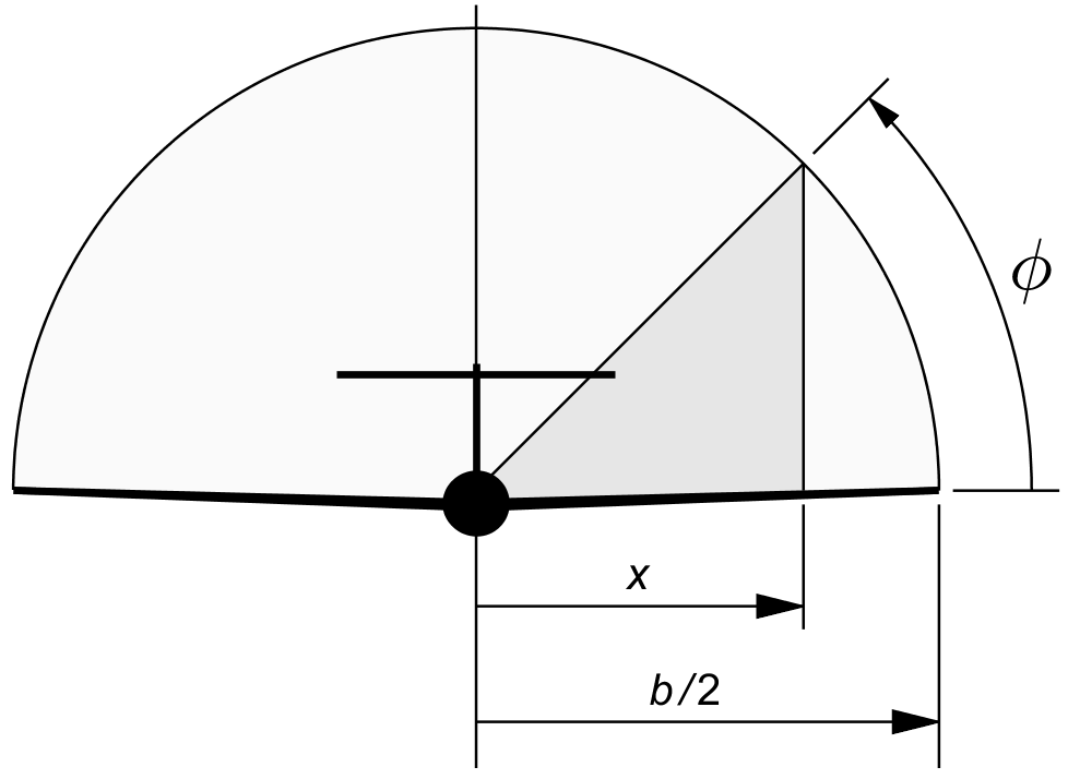
Figure 22.1 : Cosine transformation for the spanwise coordinate.
The first Fourier term for the circulation is :
| (22.2) |
The amplitude A1 can be chosen freely. It determines the contribution to the lift and the downwash for this term.
Since the combination of a cosine on the x-axis and a sine on the y-axis forms an ellipse, the first Fourier term describes an ellipse. This term represents the optimal elliptical distribution with constant downwash.
The higher order terms in the Fourier series are A2 . sin 2 φ, A3 . sin 3 φ etc. These higher frequency waves have 2, 3 etc. sine wave peaks distributed over equal distances in φ along the span, alternating between up and down inductions.
The uneven numbers give a peak in the middle and symmetrical peaks to the left and right of it. The even numbers give a zero crossing in the middle, and anti-symmetrical peaks left and right. These anti-symmetrical terms can be used to model aileron deflections and aircraft rolling motion. Using a standard sine wave integral, Glauert could show that the higher order terms do not affect the overall lift. They are just shape factors. By a more complex integral he also demonstrated that the downwash from each term has the same shape as the lift, only once divided by sin φ and with an amplitude increasing linearly with the frequency of the term. This specific integral is often called the Glauert integral.
The division by sin φ causes the downwash to increase sharply towards the tips, because sin φ is zero at the ends. The increasing amplitude with higher frequency ( i.e. , with increasing number of sine wave peaks along the span ) makes mathematical sense, since the trailing vortices are the derivatives of the bound vortex, and derivatives give sharper peaks than their base signal. The downwash for the higher order terms is much more oscillatory than the lift distribution itself.
In Prandtl's lifting line iteration, comparing the local wing sections to the Fourier terms at the same location is normally done at N points along the span, giving N control points to determine N sine wave amplitudes A1 . . AN. The control points are usually chosen at the N peaks of the highest order term. Placing them at a zero crossing would not give any information.
Only the first two or three terms of the Fourier series are smooth. The rest becomes increasingly oscillatory. The lift and downwash in between the control points is not calculated from the Fourier waves, but interpolated between the values calculated at the control points.
An alternative to assembling Fourier waves is to build up the bound vortex from discrete horseshoe functions.
Figure 22.1 shows two nested horseshoes as an example.
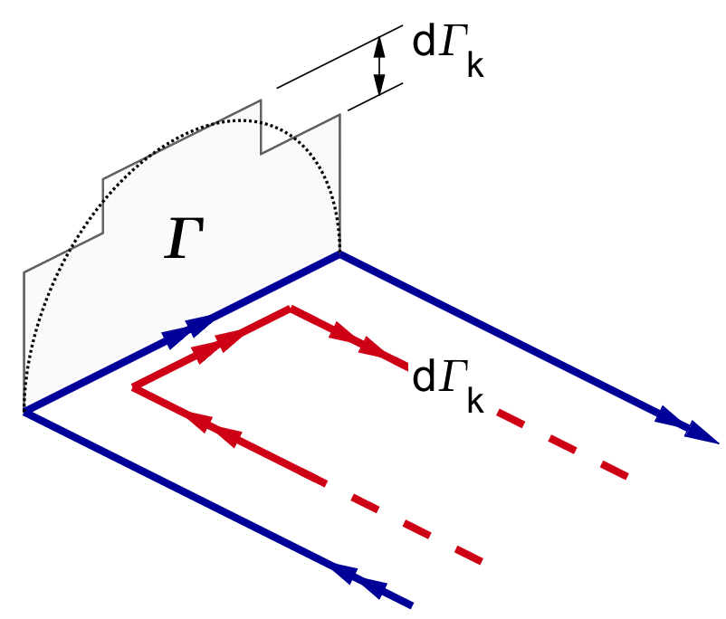
Figure 22.2 : Nested horseshoe vortices.
The resulting bound vortex is a staircase function. From figure 21.4XXXXXXXXXXXXXXXX we see that in the ellipse the bound vortex changes rapidly towards the tips. The trailing vorticity will go up sharply there, and in fact the density at the very tips it is infinite. For a limited, discrete number of horsehoes it is numerically desirable to increase the number of discrete horseshoes towards the tips.
Inspired by the cosine transformation of figure 22.1, we choose a cosine distribution for the discrete trailing vortices and for the control points. Figure 22.3 shows the idea.
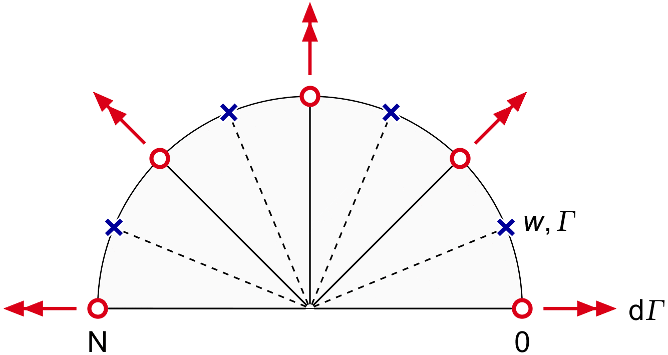
Figure 22.3 : Discrete full cosine distribution for the wing.
The trailing vortices are spaced equally over the unit circle. The control points for lift and downwash are halfway in between. This distribution is known as the "full cosine" distribution, or more formally as "Chebyshev" nodes. The N+1 trailing vortex locations xt are spread evenly from tip to tip in the angular coordinate θ :
| (22.3) |
| (22.4) |
Likewise, the N control points for the bound vortex and for the local downwash are spread evenly in the spaces between the trailing vortices :
| (22.5) |
| (22.6) |
Equation (21.6) gave the effect of a single trailing vortex at a location xt, on the downwash at a different spanwise location xw. The induction becomes infinite at the trailing vortex locations, so xw = xt is definitely not a good point to match the wing section lift to the vortex pattern. The points halfway between the trailing vortices in the angular coordinate turn out to be the perfect locations, although this seems like a minor miracle if we consider the infinite up-and-down spikes of (21.1XXXXXXXXXX) around the trailing vortex locations.
With the control points always ( "midway" ) between two trailing vortices, there are N control points between N+1 trailing vortices. The first and the last trailing vortices are at the wing tips. The total downwash at the control points xw is the sum of the contributions from all the trailing vortices at the positions xt. We will give the transfer from dΓ to dw in (21.6) the name A ( xt, xw ) :
| (22.5) |
The total downwash at a certain spanwise location xw is the sum of all the contributions of the N+1 trailing vortices d Γ ( xt ) :
| (22.6) |
If we list all the N+1 values for d Γ(xt ) along the span as a vector d Γ, then we can write this sum as a vector multiplication ( alias dot product ) of the row for xt in the matrix A ≡ A ( xt, xw ), by the N+1 vector d Γ. The result is the downwash w ( xw ) at a single spanwise location.
If we list all the local downwash values of w ( xw ) as a vector w too, then we can condense (22.6) into a single matrix multiplication :
| (22.7) |
Figure 22.4 shows how one row of the matrix A is multiplied by the vector dΓ, giving one element w ( xw ) of the vector w. Doing the full matrix multiplication gives the full transfer from the vector dΓ to the vector w.
The method can be used in the lifting line iteration between the values of the bound (and trailing) vortices and the lift that the wing section generates in the resulting downwash at the control points.
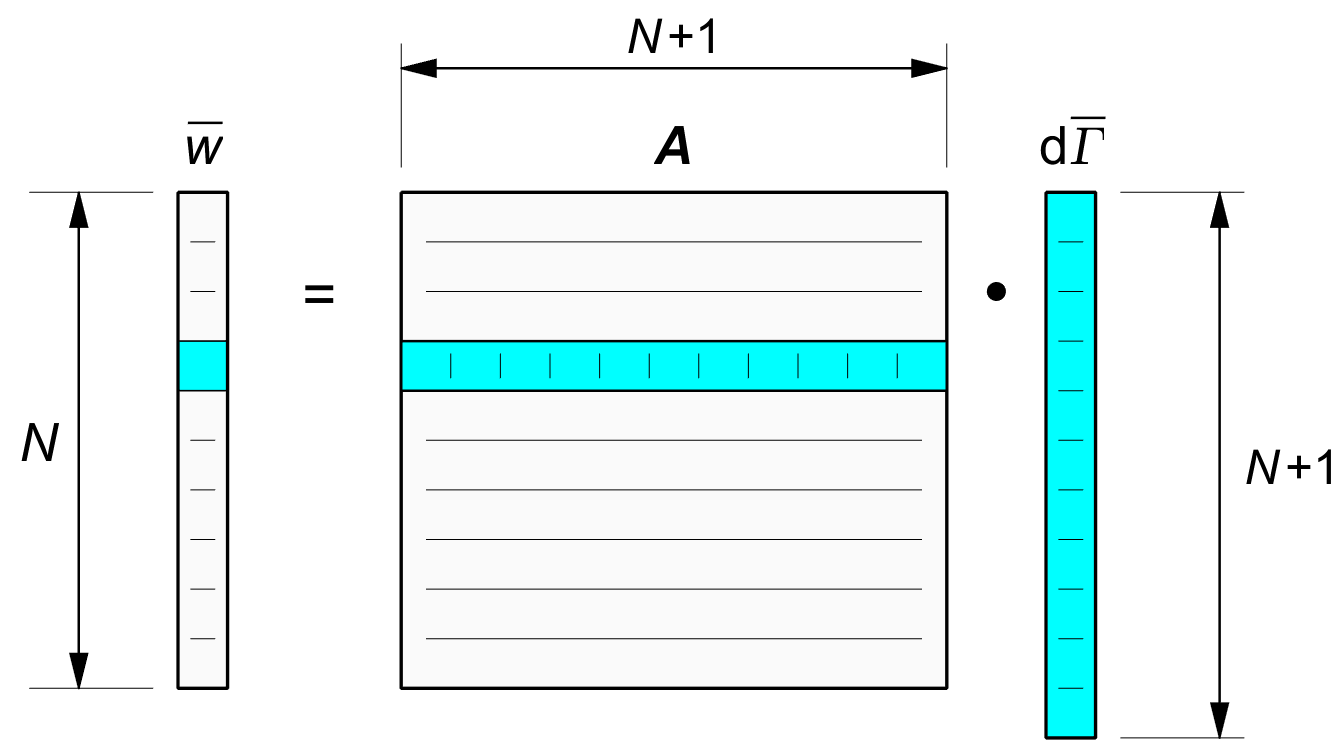
Figure 22.4 : Transfer matrix A from dΓ to w.
Equation (21.6) and the matrix A derived from it, give the downwash pattern as a function of the circulation distribution.
However, wing and propeller optimizations typically give an optimal distribution for the downwash, rather than for its "cause", the circulation. The discretized downwash pattern follows from the trailing vortices dΓ, rather than from the discretized bound vortex Γ.
If we wish to find the vector dΓ which produces the desired downwash vector w, then we must find N+1 element values for dΓ, from N element values for w.
This means we have one unknown too many, or we are one equation short. In matrix terms we can say that the matrix A has to be square before we can invert it.
We need an extra equation, and the following equality comes to the rescue :
| (22.8) |
This condition states the fact, known from potential theory, that the aircraft wing cannot create net vorticity.
All the horseshoe vortices must be closed, and so the sum of all the trailing vortices must be zero.
We add (22.8) to the matrix A by adding an extra row of 1's at the bottom. Following the rules of matrix multiplication, this adds an extra element to the end of the vector w. This extra element is not a downwash, but simply the sum of all dΓ 's. Figure 22.5 shows the matrix with this extra line added in yellow.
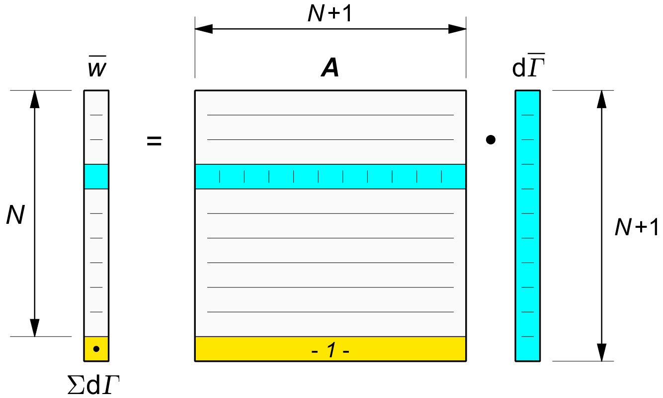
Figure 22.5 : Matrix A expanded by a row for S = Σ (d Γ ).
The resulting matrix is square, and we can solve it by matrix inversion :
| (22.9) |
Figure 22.6 shows this multiplication by A-1. To fulfil the condition (22.8), the vector w is extended by an extra element. This element is set to the desired value of the sum of the trailing vortices, which is zero.
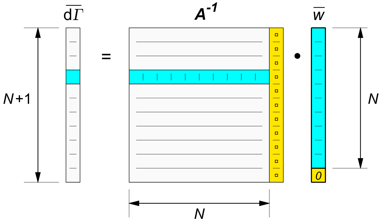
Figure 22.6 : Finding dΓ from a desired w, extended by a zero.
By the rules of matrix multiplication, the values in the final column of the inverse matrix are irrelevant, because they are all multiplied by zero, and therefore the calculation of dΓ from the actual, non-extended w in (22.9) is effectively an N+1 by N matrix multiplication. We will not be using this simplifying fact however, since in practice the matrix inverse is not explicitly calculated. Instead, (22.9) is normally solved by a more efficient Gauss elimination method. In Matlab ©, such a method is invoked by :
| (22.10) |
So far we worked with the trailing vortices dΓ at the locations xt. We now turn to the bound vortex Γ itself at the in-between locations xΓ = xw.
We know that the discrete trailing vortices dΓ are the steps in the bound vortex Γ. We will number the N+1 trailing vortices in figure 22.3 as n = 0 . . N from right to left, and the N control points as m = 1 . . N, also from right to left. The right hand tip vortex dΓo lets the bound vortex jump from zero outside the tip to Γ1 = dΓo inside it:
| (22.11) |
Each subsequent trailing vortex changes the bound vortex to the left of it by + dΓk. The incremental version of (22.11) is :
| (22.12) |
We can use this equation starting from k = 0 and ending for k = N, if we define the bound vortex strength outside the right hand tip as Γ0 = 0 and the bound vortex outside the left hand tip as ΓN+1 = 0.
In Matlab © we can write (22.12) for the vectors Γ and dΓ by the standard function cumsum() .
Equation (21.4) gave the lift for a short section of bound vortex. The total lift is the sum of all of these sections over the span. The discretized bound vortex changes only on shedding a trailing vortex, so its graph becomes a staircase plot, like in figure 22.2. This suggests integrating the overall lift by summing the constant lift sections between the trailing vortices, and this works out well.
With the trailing vortices dΓ numbered from 0 to N according to (22.3) and the vortex ( and downwash ) stations numbered from 1 to N according to (22.4), the integrated lift from (21.4) is found by :
| (22.12) |
As a verification of the inverse discrete vortex method, we run the case of constant downwash and see if it reproduces the elliptical lift distribution from the previous chapter. If successful, this is our first confirmation that Munk's analytical result.
To get a ( discretized ) constant downwash of 1, we fill the column vector w with 1's and apply (22.10).
Figure 22.7 shows the result for N = 6, i.e. for five downwash ( and bound vortex ) control points, between six trailing vortices. Together this amounts to three horseshoes. From experience, an even value for N gives nicer results, even though we already know that the center trailing vortex is zero from symmetry.
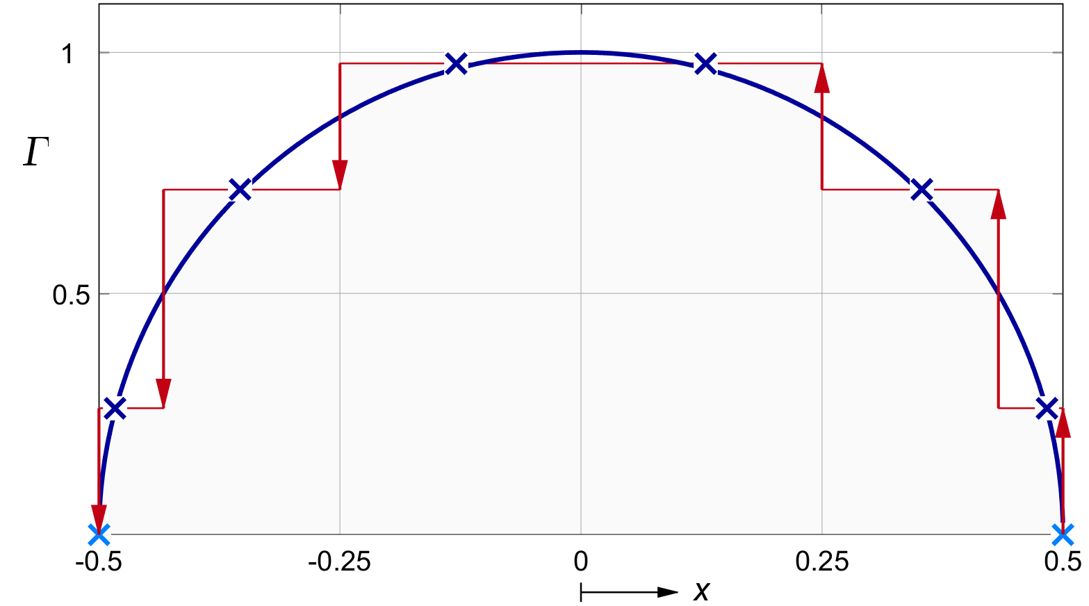
Figure 22.7 : Discretized lift for constant downwash, N = 6.
Even at N = 6 the circulation at the control points is almost spot on the ideal ellipse. At increasing N, for all intents and purposes the bound vortex points are indistinguishable from the ideal ellipse.
Remarkably, if we check the total lift by the numerical summation of (22.12), we get the exact result (21.10) of the theoretical ellipse for this downwash, for any order N ≤ 2. In other words, we get the exact result right away, even for a single horsehoe vortex :
| (22.15) |
The figure shows N = 1000 as a solid line. Even if this is not proof, it is a strong confirmation of Munk's analytical result, or viewed in the other direction, of our discretized solution.
TODO Show the downwash resulting
from the discretized circulation.
Shiver at the lines in-between the control points.