Piet Lammertse on the phase plane

The phase plane

position and velocity

The phase plane is a broad term, but we limit ourselves here to the cross-plot between the position and the velocity of a moving mass. Such a plot can be useful to get a grip on some non-linear system behaviour.

Some basic properties are :

v^{•} = a

(1)

x^{•} = v

(2)

Here x is the position, v is the velocity, and a is the acceleration of the moving mass. The dot is Newton's symbol for the derivative with respect to time. Figure 1 shows what will happen next.

The point will move to the right in the plot with the velocity x^• = v. It will move faster in direct proportion to its vertical coordinate, because that represents the velocity v. At the same time, the point will also move upward at a rate of v^• = a. The figure shows that the resulting motion has a slope of a / v.

A simple corollary is that the slope is "infinite" for v = 0. This is obvious anyway : since v = 0 means x^• = 0, a point on the horizontal axis can only move vertically away from it. In other words, the trajectories can only cross the horizontal axis orthogonally.

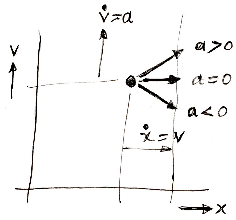
Figure 1 : Phase plane acceleration.

minimum time trajectory under a maximum acceleration / deceleration

From high school math we remember that when starting from standstill, the movement for a constant acceleration is described by :

v = a . t

(3)

x = ½ a . t^{2}

(4)

Suppose we can accelerate a mass with a maximum acceleration a_max, and maximum deceleration −a_max. Substituting t from (3) into (4) we have :

x = ½ . \frac{v^{2}}{a_{max}}

(5)

This is the equation of a parabola, but since it expresses x in terms of v, the parabola lies its side in the phase plane plot. Figure 2 shows the result. If we start from rest in the origin, then accelerate for a certain time T, and then decelerate to zero again, we will have covered a distance of x = ½ a_max T², in a time 2 .T.

Halfway, we reached a maximum velocity of v = a_max . T. For the maximum acceleration that was available, this distance could not have been covered faster. This is why this is called a "minimum time manoeuver".

The "control law", if you like, that underlies this manoeuver is : maximum to halfway, and negative maximum over the second half, starting the deceleration "just in time". This strategy is aptly called "bang-bang control". It is highly nonlinear. The phase plane method lends itself very well to the analysis of nonlinear control laws.

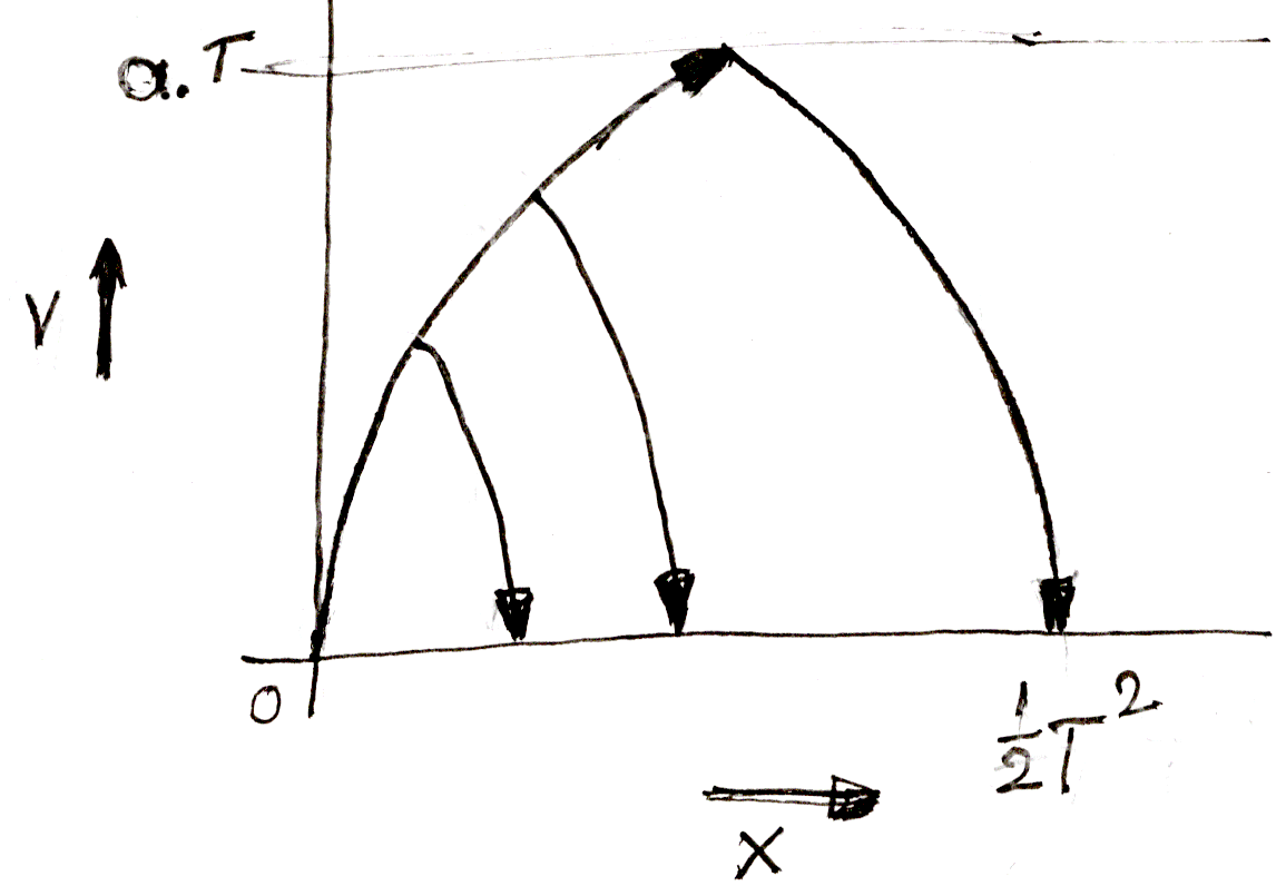
Figure 2 : Minimum time manoeuvre.

minimum time under a speed limit

Another quite common constraint is that of a maximum velocity. Taken to the extreme, we have instantaneous v = v_max, with a distance covered of x = v_max . T. This trajectory shows up in the phase plane plot as a block.

If both a maximum acceleration and a maximum velocity apply, we get Figure 3. This combines the parabolic sections of Figure 2 with a straight intermediate stretch of constant maximum velocity and zero acceleration.

This constant speed part is often called the "coasting phase". The equations are more or less obvious, if T is the coasting period.

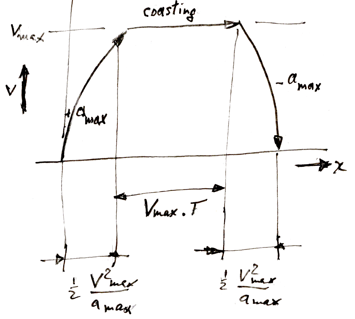
Figure 3 : Minimum time with coasting phase.

the pendulum, or mass-spring-damper system

We briefly discuss the case of a pendulum, or a mass-spring-damper system.

This is a linear system, and the phase plane plot is not very useful in this case. We discuss it only because the plot bears a superficial resemblance to the far more useful eigenvector plot, and we wish to prevent any confusion between the two.

The equations of motion for a mass-spring-damper system centered on the origin are :

m . a = − k . x - b . v

(6)

Here m is the mass, k is the stiffness, and b is the damping.

From this we see that for x = 0 :

a = − \frac{b}{m} . v @ x = 0

(7)

This shows that the vertical axis is crossed at a slope of v^• / x^• = a / v = −b / m. From (2) we concluded that the horizontal axis ( i.e. the line v = 0 ) is always crossed vertically.

This allows us to sketch the trajectory as in Figure 4. From the signs in (2), the point will always move clockwise. The trajectory is a kind of slanted spiral. We will see elsewhere that the eigenvector plot is more appropriate to this problem, and that it produces a true spiral which by convention rotates anti-clockwise.

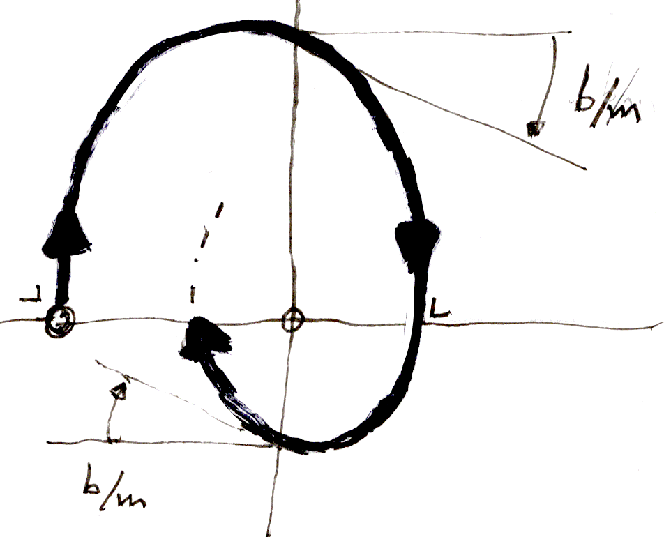
Figure 3 : Mass-spring-damper system.