Admittance control is a model-following control scheme. For the device to feel free and weightless, it must follow the model of a free floating mass. The basic model of a free floating mass is Newton's second law of motion :
| (8.1) |
For a given force and mass, the acceleration is :
| (8.2) |
The admittance controller uses the measured force as an input to calculate a model acceleration. This acceleration is based on a theoretical, imaginary mass m, which is called the "virtual" mass.
The measured force is thus interpreted as an acceleration command, with 1/< m as scaling factor, or "gain". High gain ( low mass ) gives the lightest motion, but there is a stability limit to the maximum possible gain, hence to the lowest virtual mass. When the end effector is pushed lightly, the device will start moving. When the force sensor is left untouched, the end effector will float on in a straight line until one of the device end stops is reached. A 2D device will feel like an air bearing table. A 3D device will feel like an object floating in space.
With zero damping in the virtual model, the virtual mass is not strictly passive or “stable”, in the sense that it does not come to an automatic stop. But it does not accelerate by itself either : both the position and the velocity are indifferent, or neutrally stable.
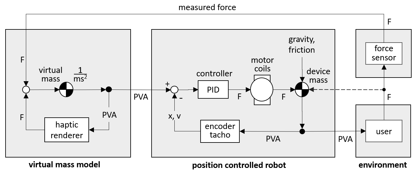
Figure 8.1 shows the admittance control block diagram. It differs from the impedance control diagram of figure 6.1 in having two nested loops, instead of just one. The inner loop is a position controlled robot. The outer loop is an "ideal" model of a virtual mass in a virtual world. This loop generates a PVA command ( position, velocity and acceleration ) command for the inner loop. This is a model-following system.
Like in figure 6.1, both the haptic renderer and the user react to displacements by forces. Contrary to popular belief, the renderer is an "impedance", exactly like it was in impedance control.
The left hand block of figure 8.1 contains the virtual mass model and the haptic renderer. Together, they completely define the reactions of the device.
The virtual mass often represents a hand held tool moving in the virtual world. Via this tool, the user interacts with a virtual ( or remote ) environment. The "haptic renderer" calculates all the reaction forces which the virtual environment exerts on the virtual tool. These forces are based solely on the position and velocity of the virtual tool in the virtual environment.
The virtual environment is an impedance. Its paradigm is : displacement in, force out.
The middle block of figure 8.1 represents a position controlled robot. This robot is simply a slave to the virtual model. It just needs to realize the calculated motions of the virtual mass.
Since there is no real hard reference for the motion of the virtual tool, the user will accept it as it is, even if it does not exactly follow an ideal model.
Do not use a velocity command and then accept what the robot makes of the integrated position, and use that in your virtual renderer.
Human perception of perceived position and velocity is not very precise, and it does not put high demands on the robot's accuracy. Provided the robot does not generate any unpleasant extra motions like sagging, bumping and vibrating, the user will not be very critical of the performance. However, like in the impedance controller, there will be stability problems when the robot fails to realize the bandwidth that the virtual model commands in a closed force loop.
This time you can have strong servo damping (or viscous damping).
TBW.
Since friction can be fully eliminated in admittance controlled devices, designers tend to accept relatively high mechanical device friction, because this allows high gearing ratios and a robust mechanical design. Such a machine cannot simulate frictionless motion in free air until it is active.
Once it is switched on, the device adopts the behaviour of a free floating mass. This virtual mass will accelerate and decelerate at the push or pull of the user, and keep floating if they no longer touch the force sensor. The robot will follow the virtual mass model, up to the frequencies that the device can reproduce. Low frequencies are like chapter 3. PVA to PVA.
Physical gravity on the end effector, and friction in the device, will not affect the feel, because these do not feed into the virtual model. Gravity is normally calibrated out of the force measurement by a zero measurement at startup of the system.
Even the direct force of the user's hand ( via the stiff force sensor ) will not affect the motion. To the position controlled robot it is just another disturbance to be cancelled. This is just as well : in the FCS HapticMaster, the virtual mass is usually set to 3 kg, while the robot inertia including the reflected inertia of the motor via a high gearing is closer to 30 kg. The direct user's push may help the motor a little while following the virtual mass, but the control loop does not really see this, or care.
At higher frequencies the picture is less ideal. The next chapter will discuss the effect of delays in the robot's response. These will affect the contact stability on stiff physical environments.
Before discussing virtual walls or dampers, we look at the software implementation of the double integrator in the left hand block of figure 8.1.
In the discrete time domain, the code which runs once every software cycle looks like this :
| (8.3) |
Here F is the sum of the forces from the force sensor and from the haptic renderer, possibly limited by a so-called PVA limiter discussed in a later chapter.
The haptic renderer force is calculated from the "current" values ofv and x, which are inherited from the previous cycle, so they in the current cycle they are really the "previous" values. The current force F is divided by the virtual mass to get the "current" acceleration. This is then used to update the virtual velocity v ( the proper term is "propagated" ). The current value of v is simply overwritten by the new one. In the last line of code, the "current" position x gets the same treatment.
Equation (8.3) looks like a simple forward Euler integrator, but there is an important difference : in Euler, x is propagated first by the current ("old") velocity. Here, we propagate it last, by the new velocity. This modified Euler integrator is called the "leapfrog", because one interpretation is that the steps in the velocity and the steps in the position take turns, like in the children's game. The "new" velocity can be interpreted as the velocity midway between the old position and the new position. In this sense, the haptic renderer calculates the "current" force F from a velocity and a position which fit moments in time differing by half a time step. It is a valid and helpful mental image, but it is best to forget it immediately.
In particular, it is important to resist the temptation to "correct" or "improve" the time difference by changing the inputs to the haptic renderer to be "at the same time". This will turn the leapfrog into a forward Euler integrator, which is highly unstable on undamped springs.
The leapfrog is a wonderfully simple implementation of the "Verlet type" integrator which was devised for astronomical and molecule simulations because it is "symplectic" : it models mass-spring-damper systems with exactly the proper damping. This same property makes it very suitable for virtual haptic rendering. In spring-like virtual force fields with no damping, the device can oscillate ( or orbit, in 2D or 3D ) for hours on end without ever diverging or converging, and the damping of virtual walls will be modelled exactly.
Unlike the impedance control renderer, the admittance control haptic renderer has perfect information about the velocity of the moving ( virtual ) mass. Using this exact velocity will give the device perfectly smooth damping.
continuous-time exponential response
The continuous-time deceleration of a damped mass is :
| (8.4) |
The theoretical response is an exponential decay, with a time constant of :
| (8.5) |
piecewise linear decay
In the discrete-time implementation of the leapfrog integrator (8.3), the decay in every time step is a straight line approximation of the exponential :
| (8.6) |
Applying these small straight line velocity steps in quick succession gives a good approximation to the continuous-time exponential, by a series of small straight-line segments.
deadbeat response
The straight-line approximation will become too coarse if the time steps get to the order of the exponential decay time. In fact, (8.5) brings the velocity to zero in a single time step when ΔT becomes equal to τ. This is called the "deadbeat" response. From (8.6), this will occur when :
| (8.7) |
At twice this damping, the velocity will oscillate between + v and − v, and for even higher values the oscillation will be divergent.
a practical damping limit
For a virtual mass of 3 kg and an update frequency
of 2,000 Hz, (8.7) yields
It is best to stay a factor of 10 away from this limit, to get a good approximation of the exponential decay. This puts the practical maximum damping at 600 [ N . s / m ], which is still extremely "stiff". It will take 6 [ N ] of continuous push force to keep the device moving at a constant velocity of 0.01 [ m / s ].
Pleasant maximum dampings for human use are on the order of 100 [ N . s / m ]. Higher values are rarely needed. Values of 10 or 30 are best for normal use.
Virtual walls are one-sided springs, with the spring force according to (6.1). The leapfrog integrator renders such springs "perfectly", i.e. with the proper damping, zero or otherwise. But the previous section showed that there is a numerical limit to the maximum damping. This also puts a limit to the attainable spring stiffness.
maximum stiffness derived from the damping ratio
A pleasantly damped spring has a so-called "damping ratio" ζ of 0.7. This non-dimensional number follows from the eigenvalues of the solution. With some manipulation the solution yields :
| (8.8) |
Typical values for the FCS HapticMaster are m ≥ 3 kg and D ≤ 600 [ N . s / m ].
With ζ = 0.7, this translates into a maximum virtual spring stiffness of :
| (8.9) |
human perception limit for the stiffness
The virtual stiffness can go beyond this value by a very large factor before going unstable, but the spring will have a bit too much damping at these larger stiffnesses. This could be corrected for by reducing the damping ratio accordingly, but in practice, K = 50,000 [ N / m ] is "infinitely stiff" to the human touch, and higher stiffness values are rarely useful.
How does it feel, 2,000, 20,000.