This chapter offers a brief introduction to closed loop control theory, since it is at the heart of all stability problems in both impedance controlled and admittance controlled haptics. Readers already familiar with control theory can skip this chapter.
Haptic devices react to the user's inputs, and the user responds to the device's outputs. This makes the device a closed loop control system, which means there is feedback going round between output and input.
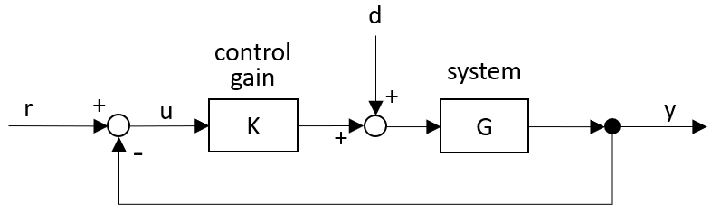
Figure 5.1 gives the block diagram for a basic closed loop control system. It has a block K which is the "controller", and a block G which is the system to be controlled. For the moment we will assume that K is just a multiplication factor, or "gain". The block G usually has all sorts of dynamics. The signal r is an outside reference. This is the moving setpoint which we wish the output y of the system to follow.
If we do not close the feedback loop, then input u to the block K will be the same as the external reference r. The "open loop" output will be :
| (5.1) |
When we close the feedback loop, the signal u going into block K changes to :
| (5.2) |
The "closed loop" output is :
| (5.3) |
The output y has become partly dependent on itself. We can bring it to the left hand side and write :
| (5.4) |
or
| (5.5) |
The mechanical systems that we are dealing with ( small robots ), will usually have a more or less fixed numerical gain of G for movements which are not too fast ( i.e., for "low frequencies" ). This will make (5.5) just an algebraic equation in real numbers. At these low frequencies, we can increase the control gain K indefinitely without running into stabilty problems. When K . G goes to infinity, the fraction in (5.5) will approach K / K = 1, which yields :
| (5.6) |
In other words, for slow motions and a very high feedback gain K, the output will follow the reference perfectly, more or less independently of the gain and dynamics of the actual system G. This is the first big advantage of feedback control.
"Disturbance" signals d, like the friction of a robot, will enter into the system G directly, not via the control gain K. Here the "forward path" in (5.4) is not K . G . u, but G . d. This changes (5.5) to :
| (5.7) |
For the disturbance d, if we let K go to an infinitely large gain, we have :
| (5.8) |
The disturbance signal has no influence on the output of the system. Its effects are completely suppressed. This is the second big advantage of feedback control.
Feedback has a downside too. It can cause instability. This instability usually takes the form of a violent, spontaneous oscillation at the maximum amplitude that the system can generate, sometimes breaking or damaging it.
Textbooks will give a formal derivation of this instability using the Nyquist criterion. A simplistic explanation of this is as follows. If the input to the system is a sine wave, there will be a frequency where the delay of the system is exactly one half of a cycle, creating the opposite peaks of the input sine wave at the output.
Entering the output as feedback into the system’s input, each peak shows up at the output again with the original sign. At this frequency, the negative feedback acts as positive feedback, delayed by one cycle. This amounts to having a plus sign on the feedback loop instead of the minus sign of figure 5.1. If we look at ( 5.7) with ( 1 - K . G ) in the denominator, then we can almost say that K has effectively become a negative number in the original equation (5.7), The feedback will increase the disturbances instead of subtracting from them them. When K . G reaches -1, the denominator becomes zero. Dividing by zero, for this frequency and gain the transfer ratio will explode to infinity. Hence, instability will occur at this gain :
| (5.9) |
It is wise in practice to stay well below this gain. Control theory defines a number of relative distance measures called "gain margin", "phase margin", "modulus margin" etc. for this. We will just remember that K . G = -1 means instability, and that we need to stay away from it.
Textbooks usually write transfer functions in terms of sine waves. The unit of frequency is called the "Laplace variable" s. This s is shorthand for a purely complex number jω , where j = √-1 and ω is the frequency in radians per second, i.e. ω = 2π f with f in Hertz, i.e. in oscillations per second.
Using math not repeated here, multiplying a sine wave by s is the same thing as taking the derivative of the sine wave. Multiplying by 1/s is the same thing as taking the time integral of the sine wave. We will use these results without proof.
Most of control theory deals with linear systems of pure differentiators and pure integrators, and the transfer functions for those are simple polynomials in s. Pure time delays unfortunately become exponentials.
There are many textbooks on control theory, often called "Feedback Control" or some similar title. They will tell this same story in considerably more detail.
Reference Franklin & Powell. Gain and phase margin, delay. Bode. Asymptotes.